Point Clouds and Blender

This blog presents a workflow on formating LiDAR derived point clouds, importing into Blender and rendering an image, utilising open source tools and data, and without the use of paid Blender plugins.

The benefits to visualising point cloud data in Blender includes realistic lighting/shading and greater control over surface characteristics of the points. Generally speaking, Blender creates nicer looking scenes.

The proposed method is suitable for small point clouds, demonstrated using a .laz dataset of around 100mb in size (8,000,000 points), resulting in a .ply output over 200mb. Please note, generating .ply files from .laz typically outputs larger sized files. Importing large .ply files (over 1gb) into Blender will take some time.

This blog assumes:

You are familiar with point cloud data, QGIS, LAStools/PDAL and CloudCompare
You have a basic knowledge of Blender, in terms of navigating, setting the camera, changing lighting, menus/toolbars, etc...

Software/tools needed:

LAStools - https://rapidlasso.de/
Download LAStools and save somewhere you can access using windows Command Prompt, cd into the LAStools/bin folder to execute commands.
LAStools offers some tools under an open license. Closed license tools employed in the workflow are fine to use for non-commercial purposes, and will slightly distort the output over a certain number of points. Review the .md or .txt doc for the relevant tool, in the relevant folder in LAStools/bin, for more information on each tool and licensing, or visit the above link.
This is the preferred tool, simply because the tools are so easy to use. Thank you rapidlasso!
PDAL (and GDAL) - https://pdal.io/en/latest/
PDAL is open source.
It is a slightly more difficult to install and use. However, it offers more functionality than any non-licensed alternative.
You need to download and install Anaconda to run the pipeline used in the tutorial - https://www.anaconda.com/
QGIS - https://www.qgis.org/en/site/
Download the LTR version.
Load LINZ Aerial Imagery Basemap as a WMTS - https://basemaps.linz.govt.nz/
CloudCompare - https://www.cloudcompare.org/main.html
Blender - https://www.blender.org/
At minimum version 3.0.
A fix for Blenders PLY import (I believe this has been fixed in version 3.6 and above. If you have the most recent version of Blender installed, can ignore this step) - https://github.com/TombstoneTumbleweedArt/import-ply-as-verts
Follow installation instructions, necessary for step 8.

Overview:

Download point cloud data
Clean and colourise a .laz file with RGB values from aerial imagery.
Convert .laz to .ply.
Import to blender.
Visualise and render an image.

1 Download data from OpenTopography

OpenTopography hosts open source point cloud data for New Zealand, under Creative Commons CC BY license. Create an account or dive on in . Download a dataset in .laz format.

Some notes:

A higher point density dataset means a more detailed final model.
You can select the 3D Point Cloud Visualizer option to view your download in 3D.
This workflow is better suited for modelling small scale areas. Pick a small area at the start to save a future hassle.

2 Clean points with LAStools

Download LAStools and save somewhere you can access using Command Prompt. In command prompt, cd to the LAStools/bin folder to execute commands. The following command will keep the point classifications of interest, and output a new .laz file. Change the -i directory to where you’ve saved your data, and the -o directory to where you want the output saved.

las2las -keep_class 1 2 3 4 5 6 17 -i C:\input\points.laz -o C:\input\pts_cl.laz

Standard classification values (ASPRS 1.4(6)):

1 - Unclassified

2 - Ground

3 - Low vegetation

4 - Medium vegetation

5 - High vegetation

6 - Buildings

17 - Bridge deck

-drop_withheld allows filtering of 1 - Unclassified points that may cause unwanted artefacts in our eventual 3D scene. Input into the command above if required.

3 Prepare imagery

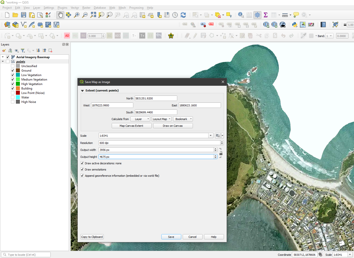
Its important to output a colour image with the same extent as your point cloud file. It is easy to do in QGIS.

Click and drag your cleaned point cloud into QGIS. Ignore the processing bar, we just want the point cloud extent to match with imagery.

Load LINZ Aerial Imagery Basemap as a WMTS service into QGIS, or use any imagery you’d like. Change the colour of the imagery by changing its brightness, contrast and saturation values in its Symbology tab, as you desire. Click Project > Import/Export > Export Map to New Image. Set the output extent to the point cloud layer (click the Layer box next to Calculate from and choose the point cloud .laz file). Set the output format as .tif. Click Save. In the next pop up, set your DPI to 300 or 600. With WMTS layers, changing the scale in your map window and setting the DPI will control the quality of your output image.

Next, perform either step 4.1 or 4.2. Each step covers a different method for colourising point cloud.

4.1 Colour points with LAStools

Run the following command to colourise the point cloud with the output image from above (change the -image, -i and -o directories):

lascolor -rgb -image C:\input\image.tif -i C:\input\pts_cl.laz -o C:\input\pts_rgb.laz -rgb

Inputs:

-rgb extracts colour channels from the image

-image is the input tif

-i is the cleaned point cloud

-o is the output point cloud

Ignore any distortion warnings that appear in terminal. For the functionality offered by LAStools, we can live with this.

To note, lascolor does not form the open source part of LAStools. It’s fine to be used for small point clouds, non-commercially. Review the lascolor.md/lascolor.txt file in the LAStools/bin folder for more information.

4.2 Colour points with PDAL

Another method for colourising point clouds is using PDAL. Use either this or the above option. First, we’ll create an environment and install PDAL (and GDAL because it’s useful). Open Anaconda Prompt and enter the following:

conda create --name lidar

conda activate lidar

conda install -c conda-forge pdal gdal

Enter y when prompted.

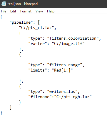
Once the above has been set up, we will next prepare the pipeline. Copy and paste the following code into Notepad/Notepad++:

{
    "pipeline": [
        "C:/pts_cl.laz",
        {
            "type": "filters.colorization",
            "raster": "C:/image.tif"
        },
        {
            "type": "filters.range",
            "limits": "Red[1:]"
        },
        {
            "type": "writers.las",
            "filename":"C:/pts_rgb.laz"
        }
    ]
}

Change the input point cloud, image and output point cloud files. Save this to a .json file, and name it col.json.

To run the pipeleine, in anaconda (with your environment activated), cd into the folder you’ve saved the .json file to, and input

pdal pipeline col.json

Which ever colourisation method used, make sure the RGB values are between 0-255 (between 1-255 for PDAL method for the Red band).

5 Load point cloud in CloudCompare

Click and drag the scaled RGB point cloud into cloud compare. Two pop up windows will appear:

Turn off all imports except for RGB and click Apply. We want to reduce the overall output .ply file size, by exporting only the minimum amount of information (We want to reduce the number of columns in our eventual .ply file).
Uncheck Preserve global shift on save, and change coordinates so that the Point in local coordinate system shows x = 0 and y = 0. Click Yes. We want to shift the X and Y coordinates to start at 0 0, and make sure this shift saves when exporting the .ply file. This is important for viewing the point cloud in Blender. If not set, the points will load well away from the centre of the workspace and is generally a pain to work with.

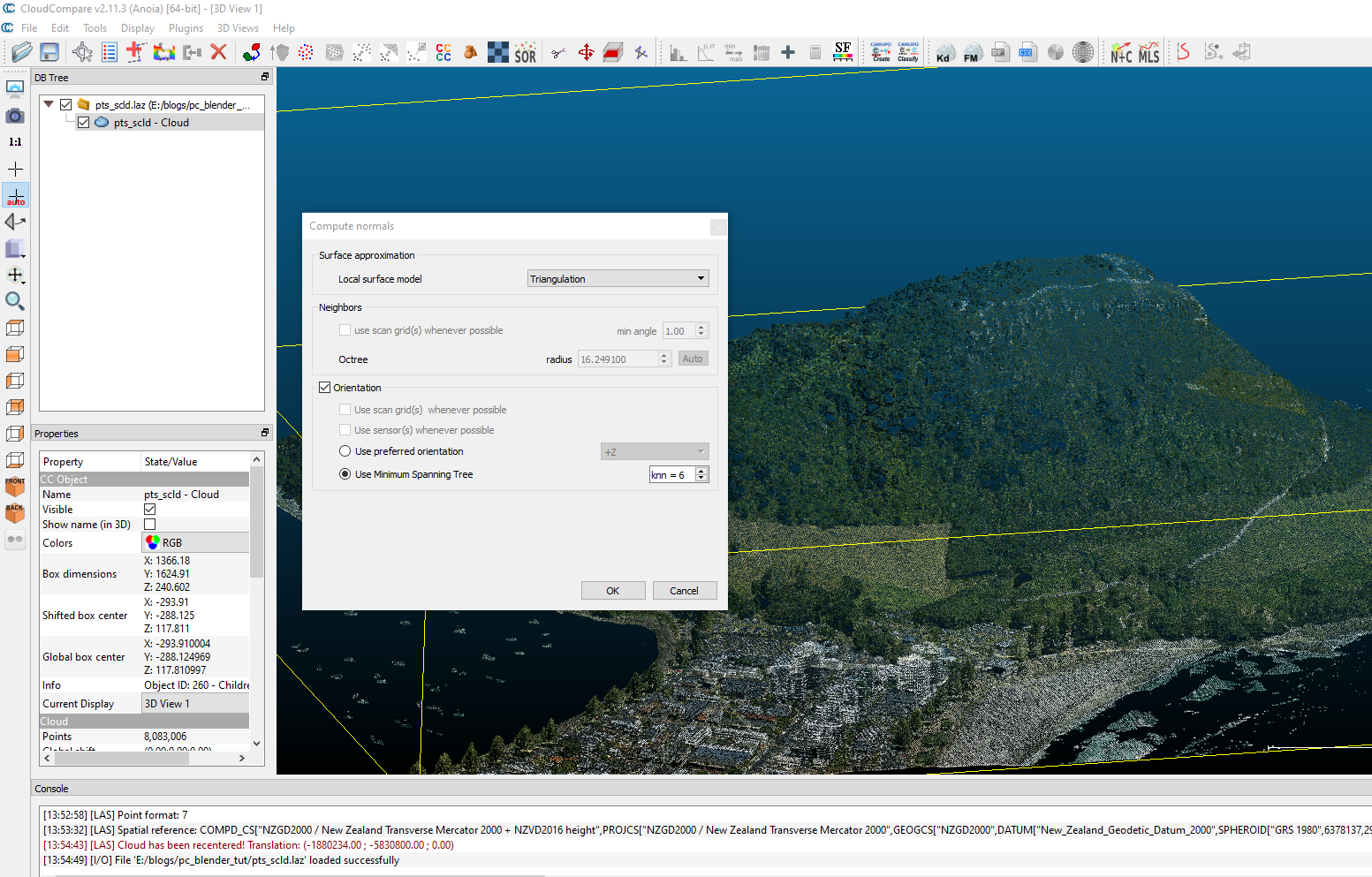
6 Compute normals

Normals, in a computer graphics context, defines the orientation of our points surfaces, and determines how they interact with light. This step is important for Blender as it will not load your imported file correctly, if not calculated.

In the top menu bar, navigate to Edit > Normals > Compute. Change Local surface model to Triangulation and click OK.

7 Save point cloud to .ply format

With the point cloud file selected, click the Save button in the top toolbar. Change the output file format to .ply. When prompted, choose BINARY.

You can view the contents of your .ply file by opening it in Notepad. You should see the following header columns:

property float x
property float y
property float z
property uchar red
property uchar green
property uchar blue
property float nx
property float ny
property float nz

8 Import .ply to Blender

Open Blender. Navigate to File > Import > Stanford PLY as Verts. If you installed the PLY import fix at the start of the blog, correctly, you should see this option in the drop down. Select the output .ply file from the earlier step. Depending on how large your file size is, this could take a while to import. You should see points now loaded in your workspace.

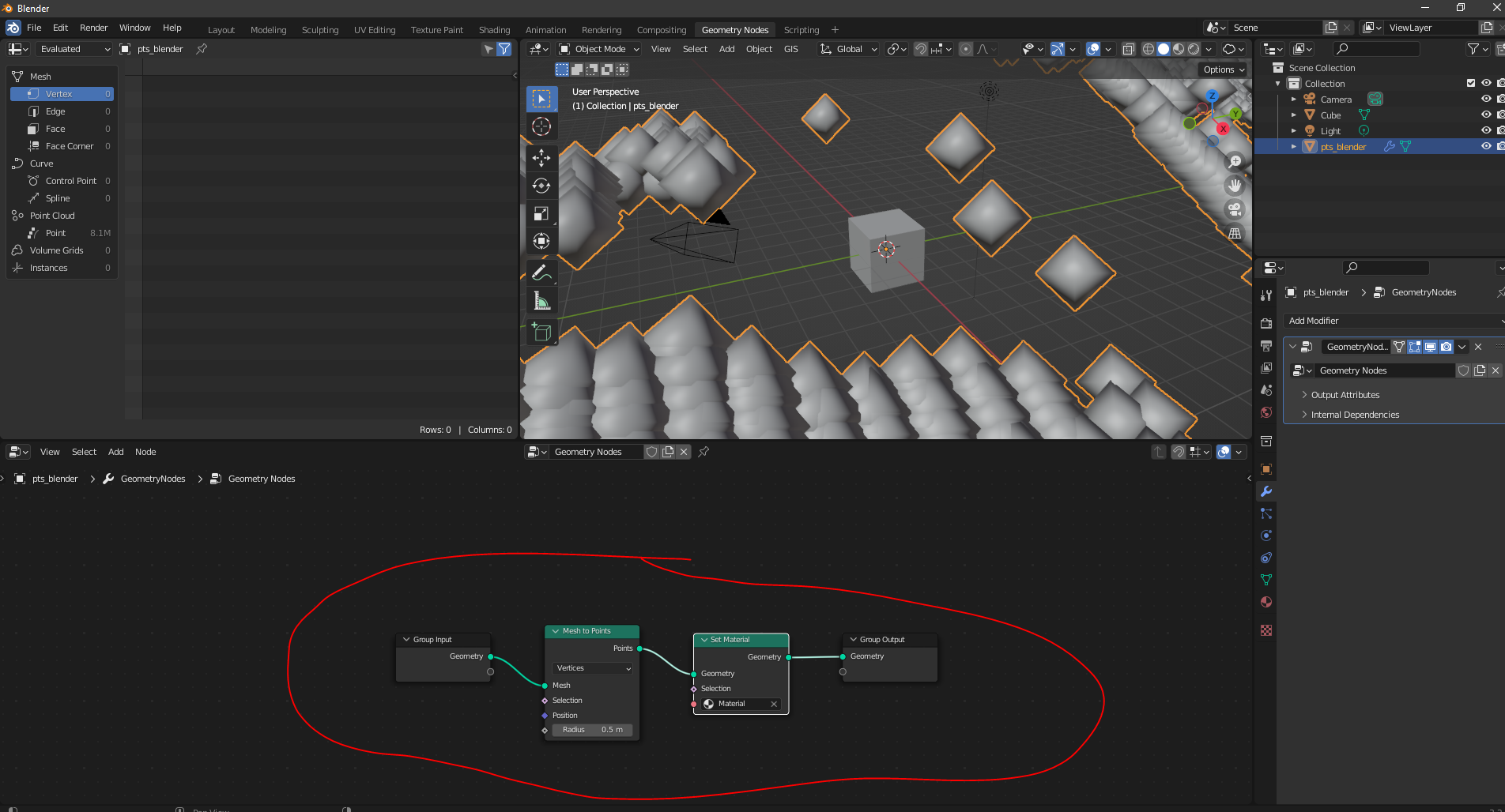
9 Set the mesh/material - Geometry Nodes tab

Select your imported points layer. Open the Geometry Nodes tab. You will know your import was successful if you see position and Col columns. These are the columns of your point cloud .ply file.Blender converts these values so ignore. Just check that the position column values are low decimal numbers (not in the millions go back to importing points to cloud compare step, and uncheck preserve global shift on save), and the Col column values are between 0 and 1. Blender changes the values and hides the normal’s columns of your imported data. Do not try make any sense of it now, research later if you want to know more.

Add two nodes, and set up as shown:

Mesh to point. Change the Radius to 0.5 (controls the point size, higher values increase point size).
Set material. In the box beneath Selection, change to Material.

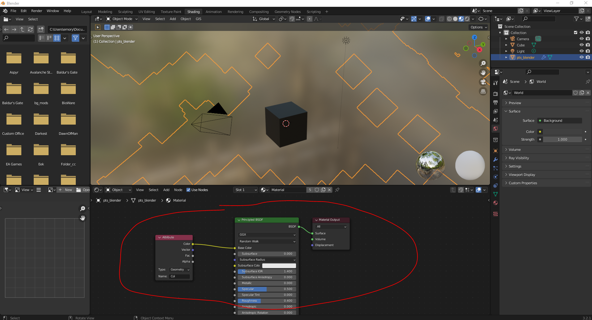
10 Set the mesh/material - Shading tab

Open the shading tab. Click the stereo-net drop down and select Material (the box just above the red circle in the image below) . Click Add and add an Attribute node. Set up as shown below. In the Name box in the Attribute node, enter the same name as the colour column you observed when opening the Geometry nodes earlier. It should be named Col by default.

11 Tweak display options

Open the Layout tab at the top of the window to go back to your scene.

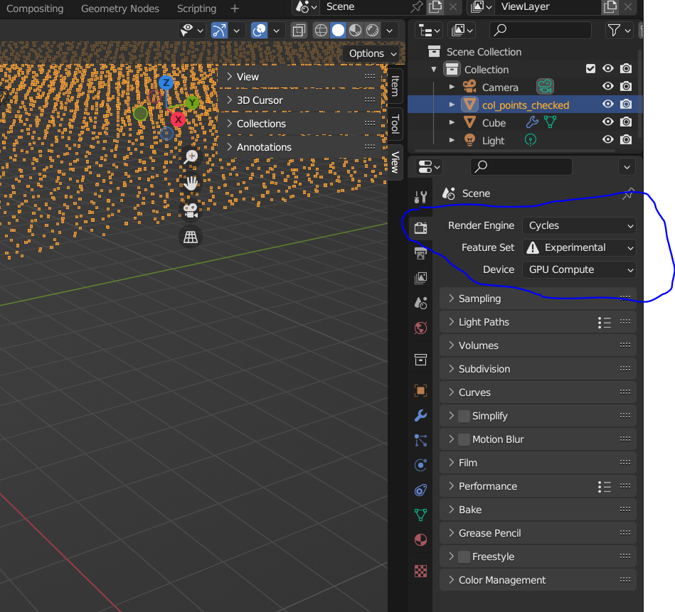
Change **Render Engine** to Cycles and **Feature Set** to Experimental (right hand side panel).

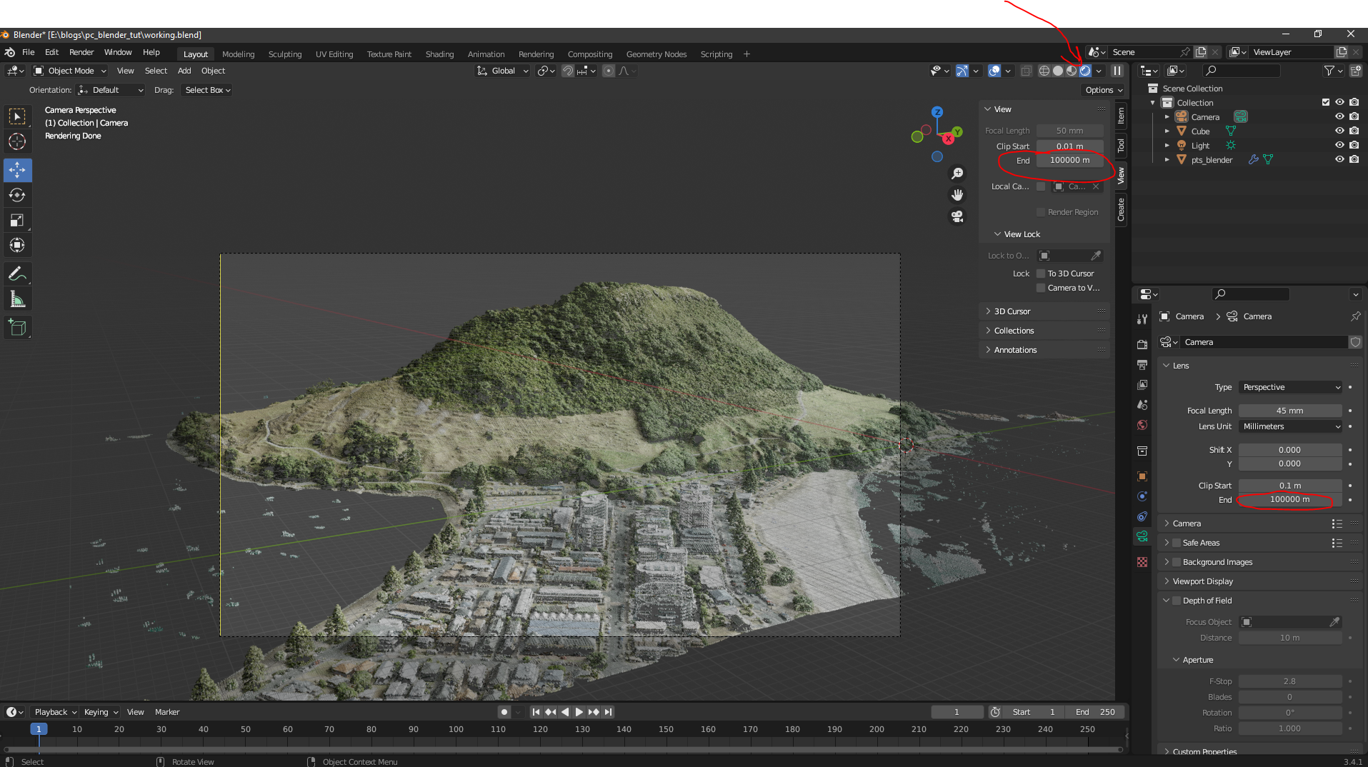
Change the View End option in both the View layout tab, and the Camera side panel, as shown circled below. A value of 100000 works. These settings control how far into the distance the 3D window and camera can view.

To view the point cloud in 3D, click the button the red arrow is pointing to in the image below. This is memory intensive. Click any of the other buttons in this row to stop rendering your scene in real time.

Use the short cut ctrl + alt = NUMPAD0 to place the camera where the current window is.

5. Click on the Light in the scene collection pane (top right). In the drop down beneath, change Point to Sun and change the following parameters:

Strength = 5.
Angle = 60.

Change the direction the sun to control the scenes overall brightness and degree of shadows, by manually moving the orange line that extends from the sun in the 3D layout window. It is a bit finicky. The sun can be moved around your 3D layout by using the Move tool (left hand side of layout window).

12 Render an image

You’re all set to render an image. Once you’ve positioned your camera, navigate to Render > Render Image.

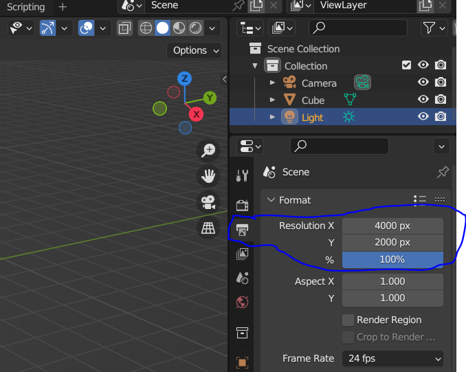
To note: change the sampling and resolution in the **Render Properties** and **Output Properties** menus increases/decreases output image render quality.

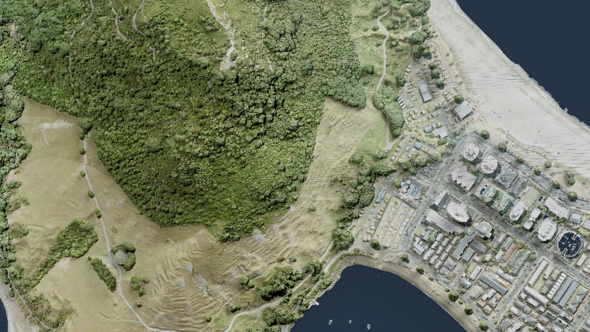
Your output could look something like this:

Thank you for reading! Hopefully you got this far and are now able to take this further than I.

Please contact info.maphustle@gmail.com if you have any questions or concerns.

Data sourced from LINZ, BOPLASS Ltd and Opentopography under creative commons CC BY 4.0